Installation
Firstly, it's recommended you have the latest version of
Python3 installed.
Python3 uses
pip3 to install packages that you'll be importing into your programs, so ensure pip3 is installed too.
Install git.
I earlier preferred not to use
Anaconda or
miniconda due to
version conflicts, unavailability of packages and dependency issues, but it's actually ok to use it. It's a good software. If any packages are missing, you can
install them. This tutorial assumes you aren't using Anaconda.
Another option is to setup a virtual environment first, because different Python packages are dependent on different versions of each other and they can cause problems with the default Linux python, which will then lead to problems with the operating system. I've found this tutorial to be good for installing and using pyenv. (Also have a look at Poetry)
Now install a bunch of peripheral packages (Not all of them are required. If you want to install just the bare-minimum, see the documentation
here):
sudo pip3 install sphinx nose networkx numpy cython pandas setuptools IPython matplotlib pylab python-tk gensim spacy
Clone PGMPy and install:
git clone https://github.com/pgmpy/pgmpy
git checkout dev
sudo python3 setup.py install
If you are wondering which IDE to use for Python, I've put up my own little review
here. I earlier preferred
LiClipse because my laptop had just 2GB RAM and LiClipse supports refactoring and autocomplete reasonably well. You could use PyCharm if you like. I now prefer VS Code (VS Code is also good enough for computers with low RAM or low processing power).
Also know about
PythonAnywhere.
Tutorial
Try creating a basic Bayesian network like this:
from pgmpy.models import BayesianModel
import networkx as nx
import matplotlib.pyplot as plt
# Defining the model structure. We can define the network by just passing a list of edges.
model = BayesianModel([('D', 'G'), ('I', 'G')])
nx.draw(model, with_labels = True);
plt.show()
If you encounter this error: "
AttributeError: module 'matplotlib.pyplot' has no attribute 'ishold'", see
this issue for the solution.
To add conditional probabilities to each of those nodes, you can do this:
from pgmpy.models import BayesianModel
from pgmpy.factors.discrete import TabularCPD
#import networkx as nx
#import matplotlib.pyplot as plt
# Defining the model structure. We can define the network by just passing a list of edges.
model = BayesianModel([('D', 'G'), ('I', 'G')])
#nx.draw(model, with_labels = True); plt.show()
# Defining individual CPDs.
cpd_d = TabularCPD(variable='D', variable_card=2, values=[[0.6, 0.4]])
cpd_i = TabularCPD(variable='I', variable_card=2, values=[[0.7, 0.3]])
cpd_g = TabularCPD(variable='G', variable_card=3,
values=[[0.3, 0.05, 0.9, 0.5],
[0.4, 0.25, 0.08, 0.3],
[0.3, 0.7, 0.02, 0.2]],
evidence=['I', 'D'],
evidence_card=[2, 2])
# Associating the CPDs with the network
model.add_cpds(cpd_d, cpd_i, cpd_g)
if model.check_model():
print("Your network structure and CPD's are correctly defined. The probabilities in the columns sum to 1. Good job!")
print("Showing all the CPD's one by one")
for i in model.get_cpds():
print(i)
print("You can also access them like this:")
c = model.get_cpds()
print(c[0])
print(model.get_cpds('G'))
print("Number of values G can take on. The cardinality of G is:")
print(model.get_cardinality('G'))
Output CPD tables:
Here, the "
variable_card" isn't about a "card". It's the
cardinality of the variable. Same with
evidence_card.
Have a look at the CPD tables and you'll see that variable cardinality for G is 3 because you want to specify three types of states for G. There's G_0, G_1 and G_2. For the variable cardinality and evidence cardinality, I feel the creators of PGMPy could've programmed it to automatically detect the number of rows instead of expecting us to specify the cardinality.
So variable cardinality will specify the number of rows of a CPD table and evidence cardinality will specify the columns. Once you've specified the CPD's, you can add it to the network and you are ready to start doing inferences.
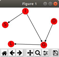
Try a slightly larger network

from pgmpy.models import BayesianModel
from pgmpy.factors.discrete import TabularCPD
from pgmpy.inference import VariableElimination
import networkx as nx
import matplotlib.pyplot as plt
# Defining the model structure. We can define the network by just passing a list of edges.
model = BayesianModel([('D', 'G'), ('I', 'G'), ('G', 'L'), ('I', 'S')])
# Defining individual CPDs.
cpd_d = TabularCPD(variable='D', variable_card=2, values=[[0.6, 0.4]])
cpd_i = TabularCPD(variable='I', variable_card=2, values=[[0.7, 0.3]])
cpd_g = TabularCPD(variable='G', variable_card=3,
values=[[0.3, 0.05, 0.9, 0.5],
[0.4, 0.25, 0.08, 0.3],
[0.3, 0.7, 0.02, 0.2]],
evidence=['I', 'D'],
evidence_card=[2, 2])
cpd_l = TabularCPD(variable='L', variable_card=2,
values=[[0.1, 0.4, 0.99],
[0.9, 0.6, 0.01]],
evidence=['G'],
evidence_card=[3])
cpd_s = TabularCPD(variable='S', variable_card=2,
values=[[0.95, 0.2],
[0.05, 0.8]],
evidence=['I'],
evidence_card=[2])
# Associating the CPDs with the network
model.add_cpds(cpd_d, cpd_i, cpd_g, cpd_l, cpd_s)
# Getting the local independencies of a variable.
print("Local independencies of G:")
print(model.local_independencies('G'))
# Getting all the local independencies in the network
print("Local independencies of other nodes:")
model.local_independencies(['D', 'I', 'S', 'G', 'L'])
# Active trail: For any two variables A and B in a network if any change in A influences the values of B then we say that there is an active trail between A and B.
# In pgmpy active_trail_nodes gives a set of nodes which are affected by any change in the node passed in the argument.
print("Active trail for D:")
print(model.active_trail_nodes('D'))
print("Active trail for D when G is observed:")
print(model.active_trail_nodes('D', observed='G'))
infer = VariableElimination(model)
print('Variable Elimination:')
print(infer.query(['G']) ['G'])
print(infer.query(['G'], evidence={'D': 0, 'I': 1}) ['G'])
print(infer.map_query(['G']))
print(infer.map_query(['G'], evidence={'D': 0, 'I': 1}))
print(infer.map_query(['G'], evidence={'D': 1, 'I': 0, 'L': 0, 'S': 0}))
nx.draw(model, with_labels = True); plt.show()
What is going on in the code:
The variable elimination queries are pretty-much self-explanatory, where you are querying for the state of a node, given that some other nodes are in certain other states (the evidence or observed variables). Inference is done via standard variable elimination or via a
MAP query. PGMPy also allows you to do variable elimination by specifying the order in which you want to eliminate variables. There's more info about this in their documentation.
What the line
infer.query(['G']) ['G'] means is that it returns a Python dict (which is like a
multimap) and then queries the key in that dict to get the value corresponding to that key (see the code below). The output looks like this:
{'G': 0}
Here, 'G' is the key of the dict, and to access the value associated with 'G' (which is zero in this case), you just have to use ['G']. So it is the equivalent of doing:
q = infer.query(['G'])
print(q['G'])
Why this tutorial
For anyone new to Python or PGMPy, a lot of this syntax looks very confusing, and the documentation does not explain it deeply enough either. The objective of this tutorial was to clear up those basic doubts so that you could navigate the rest of the library on your own. Hope it helped.
PGMPy is created by Indians, and is quite a good library for Probabilistic Graphical models in Python. You'll also find libraries for
Java,
C++,
R,
Matlab etcetera. If you want to manually try out your network model, there is an excellent tool called
SAMIAM.
More documentation for PGMPy is
here, and if you want their e-book,
an internet search will lead you to it.


